1) A brain-inspired analogy
As the term “neural network” suggests, these networks are inspired by the computational mechanism of the human brain, where each computational unit is called a neuron. While there’s very little actual resemblance between artificial neural networks and the human brain, the analogy is often used for simplicity’s sake.
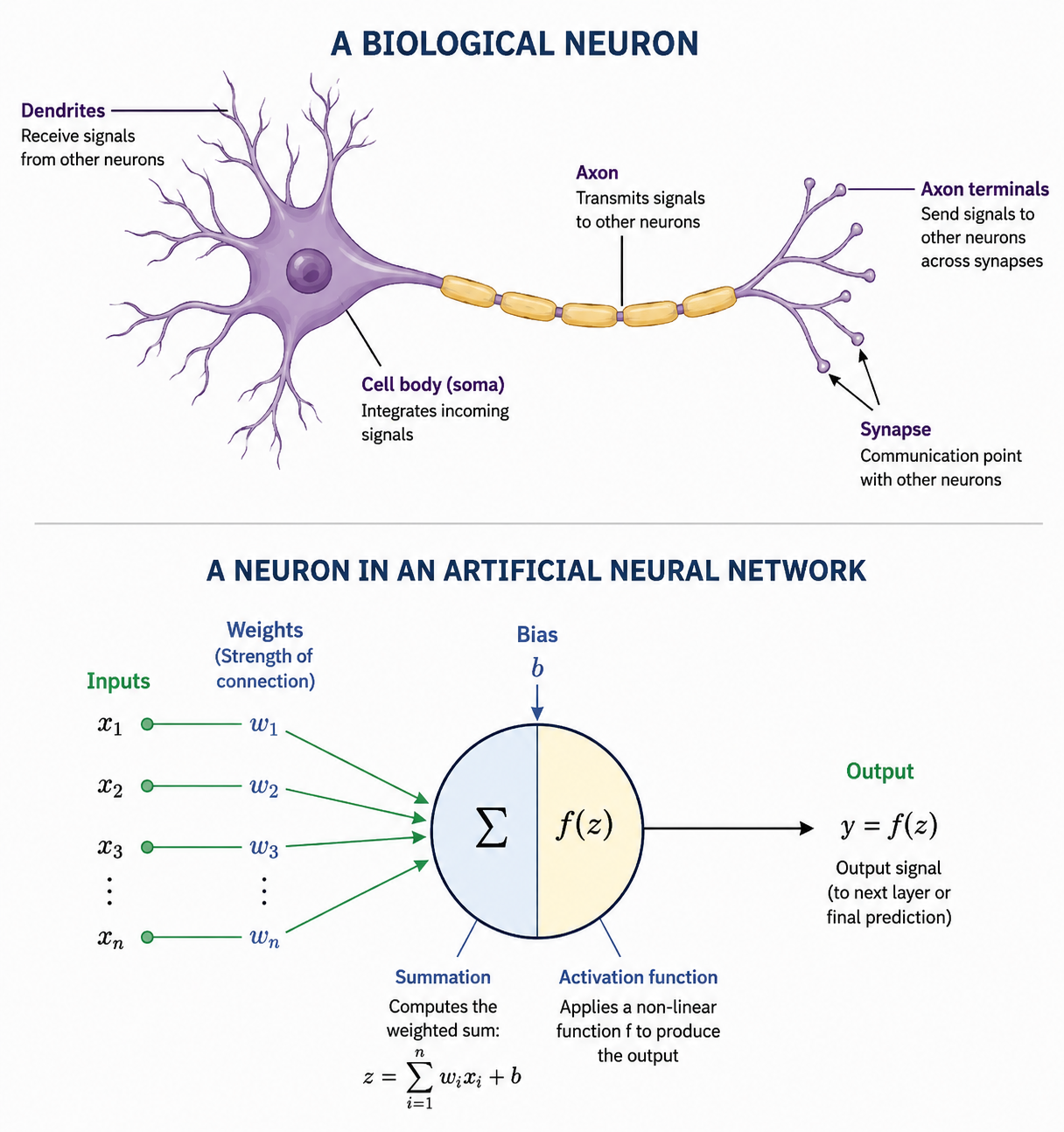 A biological neuron (top) vs. a neuron in an artificial neural network (bottom)
The neurons in our body have inputs and outputs, called dendrites and axons respectively. A neuron’s input and output are electrochemical pulses passed from one cell to another. But what we call a “neuron” in an artificial neural network is a computational unit whose inputs and outputs are numbers. What does “computational unit” mean? Look at the image above again: that circle in the middle is called an artificial neuron! The neuron’s inputs (X1, X2, X3) each have their own weights (W1, W2, W3). Each neuron multiplies its inputs by their corresponding weights, sums the results (sometimes takes the max instead), and finally applies a function f to that result before sending it to the output. Put another way, what’s happening looks like this:
$$ \text{output} = f(W_1 X_1 + W_2 X_2 + W_3 X_3) $$
where f is a step function defined as:
$$ f(z) = \begin{cases} 1 & \text{if } z > 0 \ 0 & \text{otherwise} \end{cases} $$
If the weighted sum of the inputs is greater than zero (or some threshold), the function’s output is 1; otherwise it’s 0.
The model above was first introduced by McCulloch and Pitts in 1943. They drew a connection between neurons in the human brain and logic gates (AND/OR/NOT) with binary outputs.
Frank Rosenblatt introduced a concept called the Perceptron in 1958. Rosenblatt’s idea was roughly similar to the earlier work, but what set it apart was how perceptrons learned. The problem with McCulloch and Pitts’ model was that it wasn’t capable of learning at all — it could only simulate AND/OR/NOT gates, which was considered AI at the time! Rosenblatt, on the other hand, proposed an algorithm that let the perceptron (neuron) learn. The algorithm worked like this:
- Initialize the perceptron’s weights (W) with random values.
- For each sample input in the dataset (X), compute the perceptron’s output (Y).
- If the perceptron’s output doesn’t match the label:
- If the true label is 1 but the perceptron output 0, increase the weights.
- If the true label is 0 but the perceptron output 1, decrease the weights.
- Repeat steps 2 and 3 until the perceptron makes no more errors.
Rosenblatt implemented the algorithm above on a piece of dedicated hardware and showed that it could classify simple 20×20 pixel images (keep in mind, the C programming language didn’t arrive until 1972, and he did this in 1958).
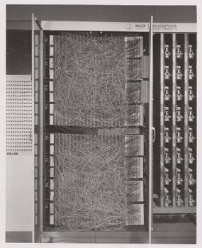 The hardware used to implement the perceptron (source: Wikipedia).
Rosenblatt’s model performed very well on binary classification tasks where the classes were linearly separable. But it performed poorly whenever the classes weren’t linearly separable.
Not long after, in 1960, Widrow and Hoff introduced the Adaptive Linear Neuron, or Adaline. They argued that the step function caused serious mathematical problems for learning (a tiny mistake could suddenly flip the output from 0 to 1, or vice versa), so they proposed replacing f with the identity function instead (the identity function just outputs whatever it’s given as input).
With that change, the perceptron’s output becomes a continuous value. As a result — unlike the step function, which wasn’t differentiable — this new function is differentiable, which opens the door to using the optimization algorithms developed in differential calculus. What Widrow, Hoff, and Rosenblatt had effectively arrived at was a form of linear regression. But what excited them most was the idea of Connectionism, which claimed:
Networks of such simple computational units can be vastly more powerful and solve the hard problems of AI.
That excitement didn’t last long. In 1969, Marvin Minsky and Seymour Papert published a book that thoroughly called perceptrons into question. One of its central criticisms was that perceptrons couldn’t learn the XOR function — or nonlinear models in general.
2) Linear vs. nonlinear models
To understand what “nonlinear function” means, let’s walk through an example. Consider the XOR function — if we plot it in two dimensions, it looks like this:
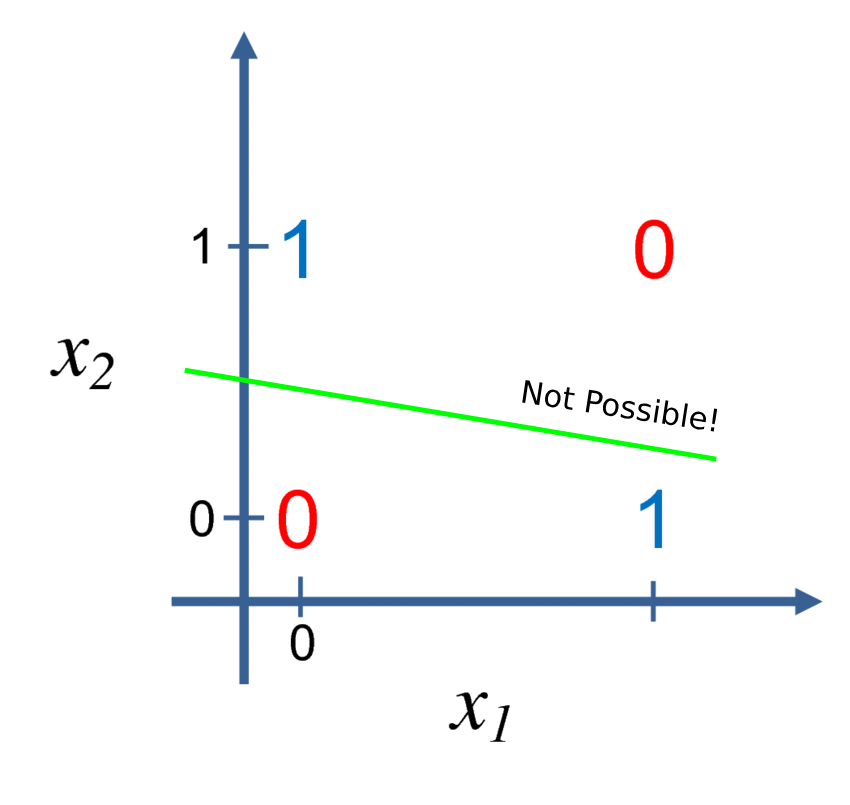 The XOR function on a Cartesian plane
Suppose we want to write a linear function f (the green line) that separates the 0 from the 1 (i.e.
draw a line with 0s on one side and 1s on the other). Since our model is linear, we’d
need to find suitable values for w and b in the line equation $y = wx + b$.
As you can see above, there’s no way to find such values that separate the 0s and 1s with a single line. Because of this, we need to use a nonlinear function that
gives us more expressive power. Take the same line equation (perceptron) xW + b. Suppose x, W,
and b are:
$$ x_1 = \begin{bmatrix} 0 & 0 \ 1 & 1 \ 0 & 1 \ 1 & 0 \end{bmatrix},\quad W_1 = \begin{bmatrix} 1 \ 1 \end{bmatrix},\quad b_1 = \begin{bmatrix} 0 \ -1 \end{bmatrix} $$
The result of the expression above is:
$$ x_1 W_1 + b_1 = \begin{bmatrix} -1 \ 1 \ 0 \ 0 \end{bmatrix} $$
If we pass the result above through a very simple nonlinear function like $f = \max(0, z)$, we get something like:
$$ \max!\left(0, \begin{bmatrix} -1 \ 1 \ 0 \ 0 \end{bmatrix}\right) = \begin{bmatrix} 0 \ 1 \ 0 \ 0 \end{bmatrix} $$
Now let’s repeat the process once more — this time feeding the previous step’s output as input to another line equation with new parameters:
$$ x_2 = \begin{bmatrix} 0 \ 1 \ 0 \ 0 \end{bmatrix},\quad W_2 = \begin{bmatrix} 1 & -2 \end{bmatrix},\quad b_2 = \begin{bmatrix} 0 \end{bmatrix} $$
Computing that line equation leaves us with:
$$ x_2 W_2 + b_2 = \begin{bmatrix} 0 \ 1 \ 1 \ 0 \end{bmatrix} $$
As you can see, we arrived at exactly what we wanted and were able to reproduce the XOR function. In other words, we used a nonlinear function like $f = \max(0, z)$ to solve XOR.
It should be clear that if we hadn’t used nonlinear functions in the example above, it would have been equivalent to just multiplying all the W matrices together (more precisely, the composition of several linear functions is itself a linear function):
$$ W_1 \cdot W_2 \cdot x = W_3 x $$
So, in order to give the network the power to distinguish between different samples (as in the example above), we’re forced to use nonlinear functions.
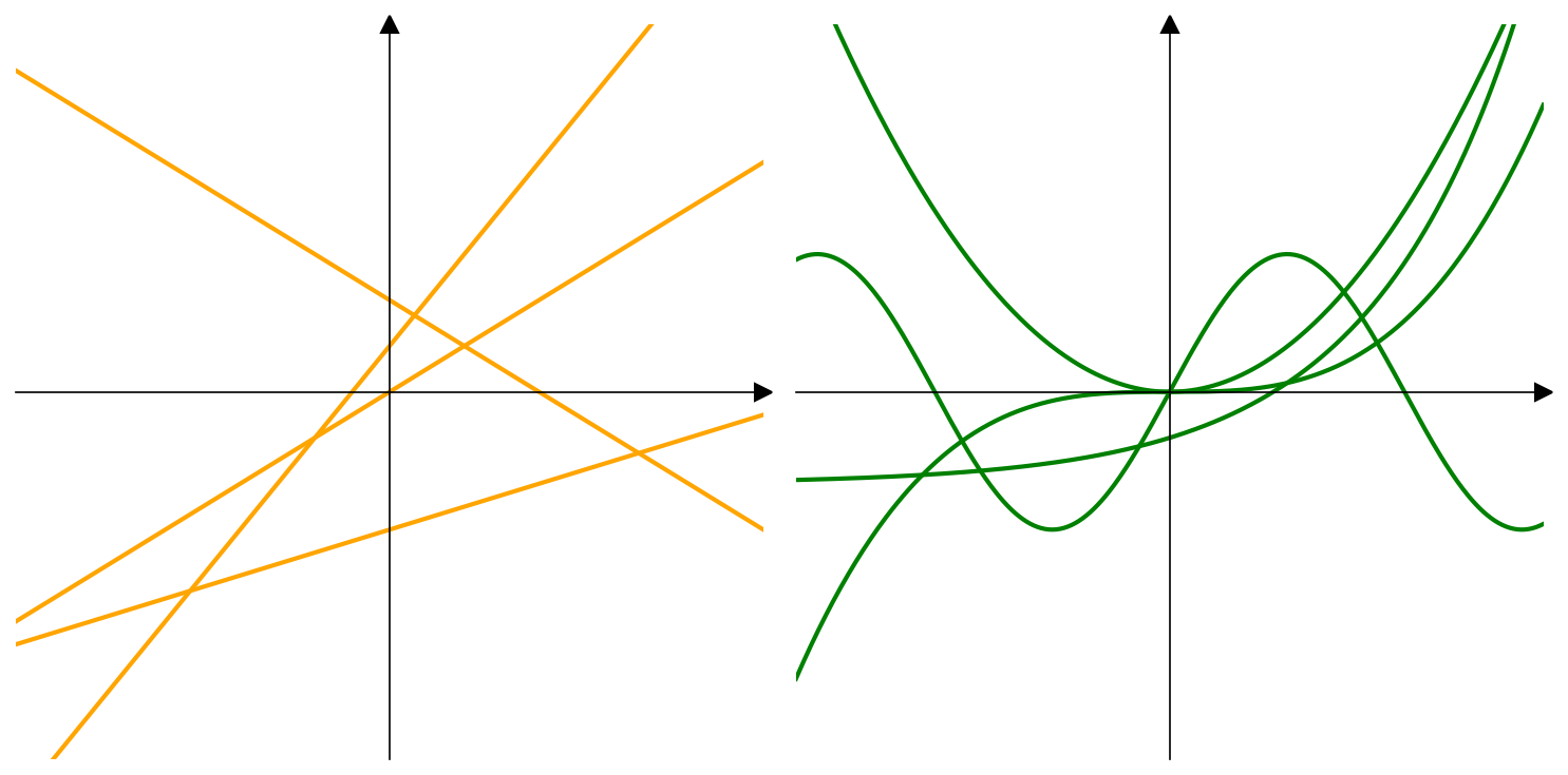 An example of a linear (left) and non-linear (right) functions
Marvin Minsky and Seymour Papert showed that: (1) the perceptron model can’t implement even simple nonlinear mathematical functions like XOR; (2) this isn’t just a limitation of a single perceptron — it’s also true when stacking multiple layers of perceptrons; (3) another issue they raised was that, even if we had multiple layers of perceptrons, there was no known way to train them. Their book was so critical that it effectively kicked off what’s now called the AI Winter, and for years afterward, hardly anyone touched neurons or perceptrons again.
That lasted until 1986, when Rumelhart, Hinton, and Williams introduced backpropagation. (In fact, what Rosenblatt had introduced earlier was, in a sense, a very simplified form of backpropagation. What we know today as backpropagation was formally introduced by these three.)
When perceptrons are connected to each other — such that the output of one perceptron becomes the input of another — a neural network is formed. In fact, a neural network is nothing more than a collection of neurons connected to one another.
3) Feedforward neural networks
Now that we’re familiar with the history of the perceptron and the definition of a neuron, understanding feedforward neural networks is fairly simple. If we let f* be our feedforward neural network, this function is nothing more than a composition of several nonlinear functions:
$$ f^*(x) = f_n(\dots f_2(f_1(x))) $$
The figure below shows an example of a feedforward neural network. Each circle in the figure is a neuron; the arrows entering and leaving it represent the neuron’s inputs and outputs, respectively. Each arrow is assigned a weight indicating how important that connection is (weights aren’t shown in the figure). Neurons are arranged in successive layers, which determine how information flows through the network. The lowest layer has no incoming arrows and is treated as the network’s input. The topmost layer, on the other hand, has no outgoing arrows and is called the network’s output. The layers in between are called hidden layers. The sigmoid symbol (∫) shown inside the neurons of the middle layers is the same nonlinear function f mentioned above, applied to the neuron’s value. In this figure, every neuron is connected to every neuron in the next layer, which is why each of these middle layers is called a fully-connected, or affine, layer.
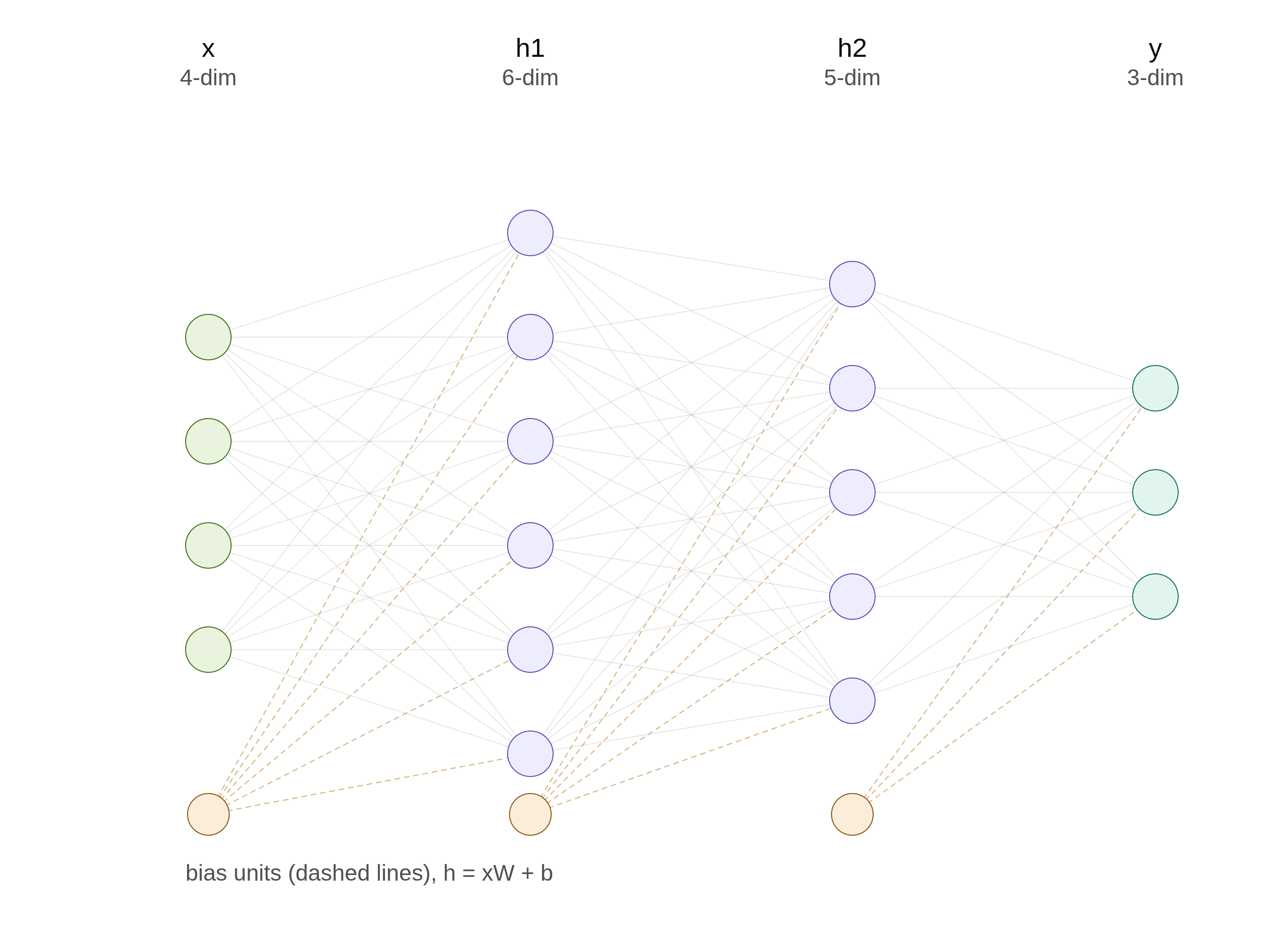 A feedforward neural network with a 4-dimensional input, two hidden layers, and a 3-dimensional output
Each layer in the network can be thought of as a vector. For example, in the figure above, the input layer (shown in green) represents a 4-dimensional vector (x). The layer above it is a 6-dimensional vector (h1), the next is a 5-dimensional vector (h2), and finally we get a 3-dimensional output vector y.
A fully-connected layer (the first one in the picture) implements the matrix multiplication h = xW, where the weight connecting neuron i in the input row to neuron j in the output is denoted W[i,j]. In other words, each circle is connected to the circle above it with a weight W[i,j]. The resulting vector h is passed through a nonlinear function g and sent to the next layer, and this process repeats for each subsequent layer.
As we saw above, the simplest kind of network is called a perceptron. It has only a single layer and can be written as a linear model:
$$ NN_{\text{perceptron}}(x) = xW + b $$
$$ x \in \mathbb{R}^{d_{in}},\quad W \in \mathbb{R}^{d_{in} \times d_{out}},\quad b \in \mathbb{R}^{d_{out}} $$
Here, W is the weight matrix and b is called the bias term. What is the bias for? As you know, we write a line equation as ax + b, where a is the slope and b is the y-intercept. A perceptron is effectively a line equation too! So what’s the point of b in a line equation?
We can build more complex networks by stacking layers on top of one another. For instance, if we add one more layer, the result is a multi-layer perceptron with a single hidden layer (MLP1):
$$ NN_{\text{MLP1}}(x) = g(xW_1 + b_1)W_2 + b_2 $$
$$ x \in \mathbb{R}^{d_{in}},\quad W_1 \in \mathbb{R}^{d_{in} \times d_1},\quad W_2 \in \mathbb{R}^{d_1 \times d_2},\quad b_1 \in \mathbb{R}^{d_1},\quad b_2 \in \mathbb{R}^{d_2} $$
Here, $W_1$ and $b_1$ are the weight and bias for the first linear transformation (layer), $g$ is a nonlinear function applied element-wise, and $W_2$ and $b_2$ are the weight and bias for the second linear transformation.
Breaking this down: $xW_1 + b_1$ is a linear transformation of the input $x$ from dimension $d_{in}$ to $d_1$, and the function $g$ is applied to each of the $d_1$ dimensions. The result then goes through a second linear transformation via the matrix $W_2$ and bias $b_2$, producing an output vector of dimension $d_2$.
We can also add yet another layer, which gives us a multi-layer perceptron with two hidden layers:
$$ NN_{\text{MLP2}}(x) = \big(g_2(g_1(xW_1 + b_1)W_2 + b_2)\big)W_3 $$
This can perhaps be written more cleanly using intermediate variables:
$$ \begin{aligned} NN_{\text{MLP2}}(x) &= y \ h_1 &= g_1(xW_1 + b_1) \ h_2 &= g_2(h_1 W_2 + b_2) \ y &= h_2 W_3 \end{aligned} $$
The vector resulting from each linear transformation is referred to as a layer, and networks with several hidden layers are commonly called deep networks.
In some cases — such as the final layer in the example above — the bias vector is replaced with 0. Question: in multi-layer networks (say, 20 layers), is the bias term actually necessary? That is, could we set every bias term to zero in a 20-layer network? I’ll leave the answer to you 🙂
4) Types of nonlinear functions
The nonlinear function mentioned above is known in the neural network world as the activation function, and it can take many different forms. There’s currently no strong theory for which type of nonlinear function to use, and choosing an appropriate one is often done empirically. Below, we go over two nonlinear functions commonly used in earlier work: sigmoid and the rectified linear unit (ReLU).
Sigmoid: The sigmoid activation function $\sigma(x) = \dfrac{1}{1+e^{-x}}$, also called the logistic function, is an S-shaped function that squashes each element of vector x into the range [0, 1]. Since the early days of neural networks, sigmoid has been one of the standard nonlinear functions in this field, but it’s now largely deprecated for internal layers in favor of the functions below, which tend to perform better.
ReLU: The ReLU activation function, also known as the rectified linear unit, is an extremely simple activation function that’s easy to work with and produces good results in most cases. It maps every value x < 0 to 0. Despite its simplicity, it performs remarkably well across a wide range of tasks.
5) The power of feedforward networks
Prior research has shown that neural networks have very high computational potential. Given enough neurons, a nonlinear function, and properly tuned weights, they can approximate a wide range of mathematical functions — this is why they’re referred to as universal approximators. What does that mean? It means that if we have a feedforward neural network with enough neurons, and we can find suitable weights for it, then we can approximate a broad range of mathematical functions.
A reminder: “approximate” means reaching a result close to what the true function would give us, within some margin of error. You might ask, what’s the point of approximating? Many mathematical problems have exponential (or worse) complexity — they’re in the NP-Hard class. Think of the 0-1 knapsack problem, or the traveling salesman problem. There’s currently no known algorithm that solves these problems in polynomial time, but with a good approximation algorithm, we can find a solution close to the optimal one.
Theoretically, it’s been shown that MLP1 is a universal approximator. This might suggest that there’s no need to go beyond MLP1 to more complex architectures. But the catch is that these theoretical results say nothing about how to learn the network’s weights (the theory claims such a network exists, but says nothing about tuning its parameters given training data). It also says nothing about how large the hidden layer needs to be! Because of this, in practice we use neural networks with relatively small layers (at most a few thousand units), and we train them on a relatively modest amount of data using local search methods like stochastic gradient descent. Since the theory above offers no guarantees under these non-ideal, real-world conditions, it’s often better to use architectures more sophisticated than MLP1 — though in many cases, MLP1 still gives very good results.
In other words, we might have an MLP1 network with 100 neurons that solves our task, but that same MLP1 could be converted into an MLP2 network (an MLP with two hidden layers) — with 11 neurons in the first layer and 9 in the second — and achieve the same accuracy as the original MLP1. In effect, we get comparable accuracy with roughly 1/5 of the neurons, and that’s exactly why deep networks are so widely used.
6) Miscellaneous
As we’ve seen, the output of a neural network is a $d_{out}$-dimensional vector. When $d_{out} = 1$, the network’s output is a single scalar value. This kind of network can be used for regression (or scoring) problems, or binary classification. Networks with $d_{out} = k > 1$ can be used for k-way classification problems.
The matrices and bias terms used to define linear transformations are called the network’s parameters. We usually denote the full set of network parameters as $\theta$.