At a high level, modern transformers take an input (text, image, voice) and generate an output (text, image, voice). Simply put:
| |
Tokenizer
We skip explaining the tokenizer piece here, because the goal of this post is the
transformer itself. The tokenizer converts raw text into a sequence of ids (using
encode()):
"What's your name?" -> [13347, 885, 634, 1308, 30]
The pretrained transformer model generate a output_idx and tokenizer again converts a sequence of ids back into raw text (using decode()):
[13347, 885, 634, 1308, 30] -> "What's your name?"
A basic transformer
Let’s start with a basic (GPT-2-style) transformer class. I skipped dropout, tensor reshaping/transposing, and some other details for brevity.
Generally, a transformer decomposes into multiple pieces such as embedding layers, attention layers, feed-forward layers. Modern transformer architectures usually differ from each other by:
a) how they implement embeddings (e.g. to support larger context — 1M tokens), b) how they implement the attention mechanism (Multi-Head Attention, Grouped-Query Attention, Linear Attention, etc.), c) how residual connections, layer norms, and feed-forward layers are arranged across layers, and d) other innovations such as KV-caching, the optimizer, or the activation function.
Let’s look at the original transformer with Multi-Head Attention (MHA):
| |
Multi-Head Attention
Probably the most important piece is the attention block, which we can write as:
| |
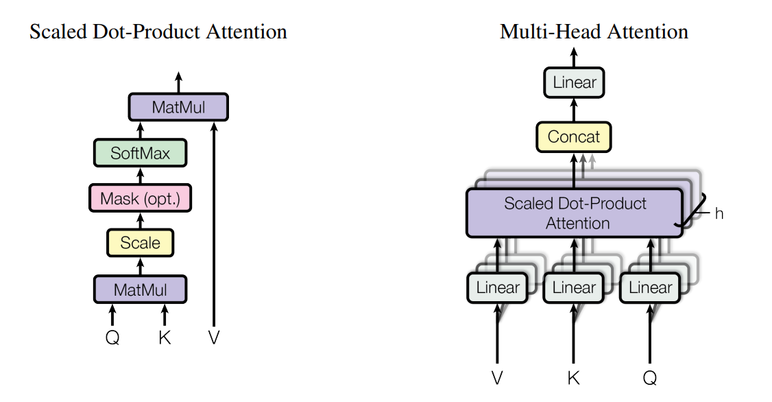 Multi-Head Attention
Reducing the memory bottleneck
The above architecture has a severe bottleneck: memory bandwidth overhead at decoding time. This is where the interesting design space opens up — the goal becomes reducing this memory bottleneck, and several solutions have been proposed to do it.
Grouped-Query Attention
One solution is Grouped-Query Attention:
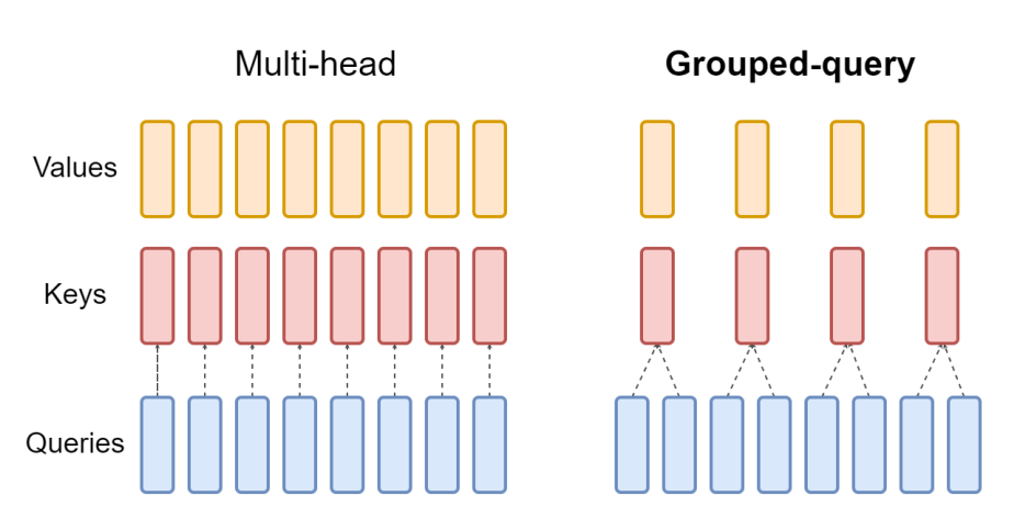 Grouped-Query Attention
Grouped-query attention divides queries (q) into G groups, each of which shares a single key (k) and value (v). Basically:
| |
As you can see, instead of three linear layers (self.q_proj, self.k_proj, self.v_proj) of size hidden_dim * hidden_dim, we have
two smaller linear layers (self.k_proj, self.v_proj) whose size is determined by n_kv_groups.
This reduces the size of the k/v projection (1024×512 instead of 1024×1024) and, more importantly in practice, the size of the kv cache during decoding (8 kv heads stored instead of 16).
What is the KV cache?
As the name suggests, it’s about caching k and v values and reusing them later in the process. You might ask why. As you know, we generate one token at a time during decoding:
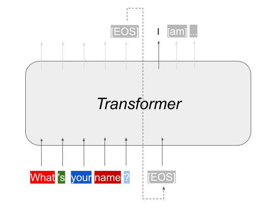 Transformer decoding, one token at a time
During decoding, we have to wait and see what token we generated previously in order to generate the next one. What happens is a loop:
| |
We generate one token after another and feed the concatenation back to the model until we
reach a specific token — an end-of-sequence marker, here assumed to be 0.
As you can see in this while-loop, for every new token we want to generate, we pass the
entire sequence (input_idx) and recompute all the attention and linear layers. But we can
cache part of that computation to avoid repeating it. That’s where KV-caching comes in.
KV-caching has two phases:
Prefill: we feed the initial input_idx (our prompt, “What’s your name?”) to build the
initial KV cache.
Decoding: we feed one token at a time and reuse the already-computed KV values in the cache.
Our while-loop then becomes:
| |
We pass a new argument to transformer.__call__ (kv_caches). Looking back at the
transformer class:
| |
The important part is the attention mechanism though:
| |
Note that above, instead of passing the entire sequence ([13347, 885, 634, 1308, 30]) for
a new token, we only compute projections on the last single token. Then, to calculate
attention, we reuse the cache. The attention function, instead of computing q_proj,
k_proj, v_proj on the full sequence of length 5, computes them on a single token.
Skipping that computation means fewer matrix multiplications and a faster response time.
Ask yourself: why don’t we cache the query (q)?
However, this useful caching mechanism comes at a cost: memory bandwidth, as briefly mentioned above. As sequences grow, storing the cache becomes increasingly expensive. For example, a large input prompt of 10,000 tokens requires storing ~491.5 MB in memory (2 [for K and V] × 12 [number of layers] × 10,000 tokens × 1024 [hidden size] × 2 bytes [fp16] = 491,520,000 bytes ≈ 491.5 MB) — and that’s just the KV cache, before accounting for the rest of the transformer’s computations. In model deployment, this KV cache is a major bottleneck that limits the maximum batch size and sequence length.
At batch=128 (a realistic serving batch), we’re already at ~63 GB — more than an A100/H100’s 80 GB, leaving almost nothing for the model weights themselves. Note that our 12-layer, 1024-hidden config is small — a real 70B model has ~80 layers and ~8K hidden dim.
Multi-Head Latent Attention
As we saw, Grouped-Query Attention reduces the computation requirements. But DeepSeek-V2 claimed that the downstream task performance of Grouped-Query Attention is inferior to original Multi-Head Attention, and introduced Multi-Head Latent Attention instead.
Instead of sharing KV heads across groups, it compresses (down projection) k and v into a smaller vector for each token, caches that (a much smaller vector than the full k/v), and reconstructs (up projection) the full-size k/v from the compressed vector on the fly. This keeps a much smaller cache. Specifically:
| |
As you can see above, they compressed x down to a smaller size (via self.kv_down_proj) and only
cache that. When needed, they reconstruct it via self.k_up_proj and self.v_up_proj — we
reduce the KV cache (memory) at the cost of higher compute. Why is that a good trade? Because
at decoding (inference time) we’re memory-bound rather than compute-bound. It means, the GPU spends a
lot of time moving data, in & out of GPU’s memory VRAM, rather than doing actual computation (matrix
multiplication). We have lots of memory in VRAM but we have only a few kilobytes of register space.
VRAM (GB) -> L2 Cache -> L1 Cache -> Registers (KB) -> Tensor-core (actual computation happens here!)
Now let’s assume you want to move a 1024x1024 matrix into the tensor-core — that means moving 1024*1024 ~= 1 million elements, roughly 1M x 2 bytes = 2MB, which is already far larger than the register space!
In the next post in this series, I’ll cover some other tricks used in modern transformers to work around this memory bottleneck.