When we work with textual data, we’re often dealing with a sequence of characters, words, or sentences, and in most cases the order of that sequence matters to us. Recurrent networks in theory let us represent a sequence of unknown length as a fixed-size vector, while still preserving many of the syntactic and structural properties of the input sequence.
Simply, a Recurrent Neural Network (RNN) can be seen as a function that takes an input of length $n$ (e.g., assume a sequence of words) and returns an output vector $y$ of dimension $d_{out}$:
$$ \text{RNN}(x_{1:n}) = y, \qquad x_t \in \mathbb{R}^{d_{in}}, \quad y \in \mathbb{R}^{d_{out}} $$
Here $x_{1:n}$ is our input sequence, where each word has been mapped to a vector of size $\mathbb{R}^{d_{in}}$. These vectors are fed as input to the RNN, which returns an output $y$. More precisely, the output is $y_{1:n}$, but we often only care about the last state, $y_n$. Why? Because it somehow carries information about all the previous words. So we simplify and drop the subscript, calling it $y$.
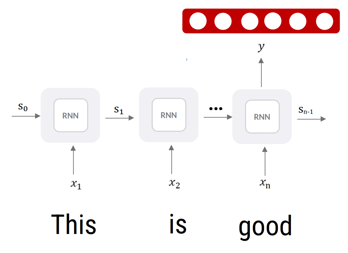 The sentence “This is good” fed into an unrolled RNN
In the example above, the sentence “This is Good” is fed into the recurrent network, producing an output vector (shown in red). This vector — sometimes called a feature vector, since it’s representative of the linguistic and syntactic features of the input — can be used for other tasks like sentiment analysis. For example, we can feed the output vector to an MLP classifier, and the network predicts the sentiment probability of the input document based on that.
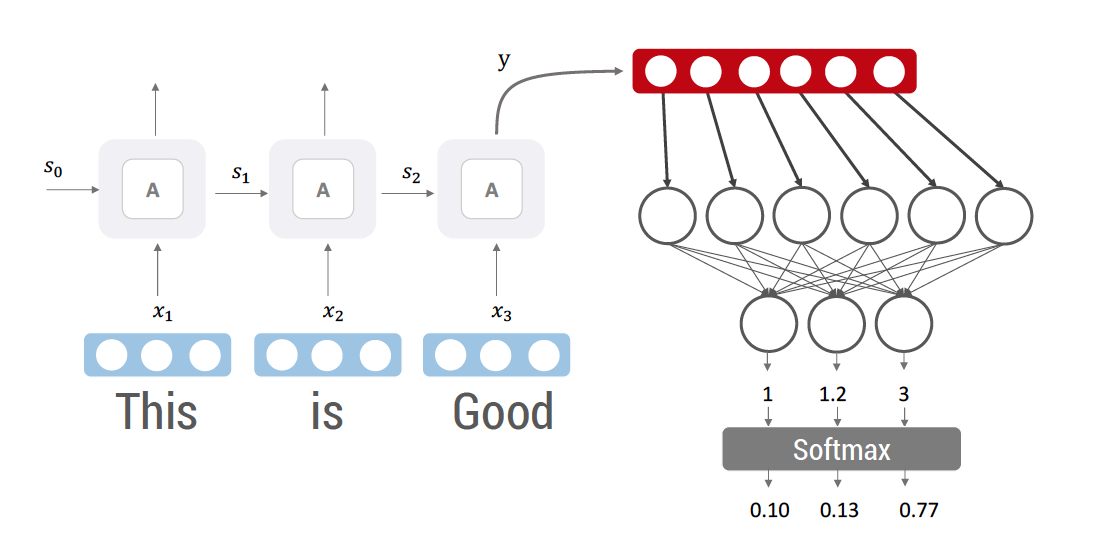 The RNN’s output fed into an MLP classifier to predict sentiment
Why recurrent?
Now, why are they called “recurrent”? There’s nothing visibly recurrent in the figure above, so where does the name come from? If we state the formula above a different way, we can define any recurrent network as follows:
$$ \begin{aligned} \text{RNN}^*(x_{1:n}, s_0) &= y_{1:n} \ s_t &= R(s_{t-1}, x_t) \ y_t &= O(s_t) \end{aligned} $$
This says that every recurrent function is made up of two main parts: a recurrent part, denoted $R$, and an output part, denoted $O$, whose job is to produce the output vector $y_t$. In fact, how we choose to define these two functions determines the type of recurrent network we have in literature (e.g., SimpleRNN, LSTM, GRU, …).
The state vector $s_t$ can be thought of as a kind of memory that stores information from previous steps. More precisely, $R$ takes the state vector from the previous step $s_{t-1}$ and the input vector $x_t$, and returns the next state vector $s_t$ (the initial state $s_0$ is usually initialized to zero or some random values). You can think of it as a memory that starts out empty and, over time, gets updated with a bit of knowledge from each new input.
The output of $R$ (i.e., $s_t$) is then turned into the output vector $y_t$ by another function, $O$. Depending on the architecture, $O$ could be different, or, as we’ll see for SimpleRNN below, nothing at all (identity function).
So the figure above is really the recurrent network unrolled over time; in its non-unrolled (folded) form, it looks like this:
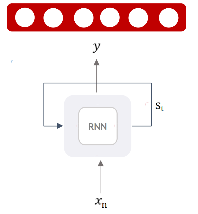 The folded (non-unrolled) view of the RNN
Inputs are fed into the network one at a time — at each time step, a single word $x_t$ is given as input, producing an output and a state vector $s_t$.
Inside the cell
Now that we have some intuition for the RNN, let’s look inside and see how it actually works.
As mentioned above, the cell takes two inputs: the input $x_t$, and the state vector from the previous step, $s_{t-1}$. What happens inside is a few vector-matrix multiplications and addition. For SimpleRNN specifically, we can write:
$$ \begin{aligned} \text{RNN}^*(x_{1:n}, s_0) &= y_{1:n} \ y_t &= s_t \ s_t &= \tanh(s_{t-1} W_{s} + x_t W_{x}) \end{aligned} $$
The RNN takes a sequence of vectors $x_{1:n}$ and an initial state vector $s_0$, and returns the output $y_{1:n}$. The output $y_t$ is simply the state vector $s_t$ — here $O$ is the identity function, so no separate transformation is applied to get the output.
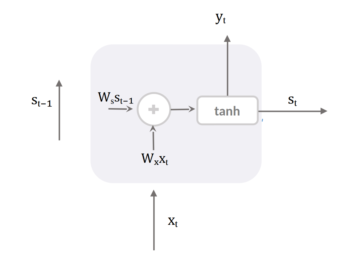 Inside a SimpleRNN cell
The state vector $s_t$ is obtained by multiplying the previous state vector $s_{t-1}$ and the input vector $x_t$ by their own weight matrix ($W_s$ and $W_x$ respectively), summing the results, and then applying the hyperbolic tangent — tanh normalizes values to the range $[-1, 1]$ (the initial state vector $s_0$ is filled with a default value, and together $W_s$ and $W_x$ make up the full weight matrix $W$).
A toy implementation
If we wanted to write a piece of code for what’s described above, it would look something like this:
| |
Everything above describes SimpleRNN, the simplest kind of recurrent network. Depending on how we define the $R$ and $O$ functions, we get different types of recurrent networks (LSTM, GRU, …).
The problem with SimpleRNN
SimpleRNN has a serious weakness: it struggles to carry information across long sequences. At every step, the state vector $s_t$ passes through a $\tanh$ and gets multiplied by the same weight matrix $W_s$ again. Over many steps, this repeated multiplication tends to either shrink the gradient toward zero or blow it up, depending on the values in $W_s$ — the well-known vanishing/exploding gradient problem. In practice, this means SimpleRNN has a hard time learning dependencies between words that are far apart in a sequence (imagine needing to connect a pronoun at the end of a paragraph back to a name mentioned in the first sentence).
This is exactly the problem LSTM and GRU were designed to fix. Both replace the simple add-then-tanh update of SimpleRNN with a more deliberate mechanism — gates that control what gets written into the state, what gets forgotten, and what gets passed through unchanged — which makes it much easier for gradients (and information) to flow across long sequences. We’ll look at how those gates work in a future post.